
Modeling Wave and Seabed Energetics on the California Continental Shelf
By Li H. Erikson, Curt D. Storlazzi, and Nadine E. Golden
Chapter 1. Introduction
Background and motivation
Ecologists have long recognized that the structure and function of benthic marine ecosystems are closely linked to oceanographic processes (Mann, 1973; Graham and others, 1997; Snelgrove and Butman, 1994); most studies, however, have relied either upon qualitative descriptions of oceanographic factors (such as, “low”, “medium”, or “high” energy environments) or on quantitative values based on mean oceanographic conditions (e.g., tidal range or wave heights). Recently, the importance of intermittent disturbance on marine habitats has been addressed by Thrush and Dayton (2002), Roff and others (2003), and Goodsell and Connell (2005) among others. These studies show that quantifying the natural spatial and temporal variability of disturbances affecting benthic marine ecosystems can be critical for managers and planners tasked with forecasting the effects of particular management practices such as marine protected areas. Understanding the natural variability of sea floor disturbance is also critical for local, State, and Federal agencies responsible for permitting offshore activities such as trawling, dredging, and the placement of sea-floor engineering structures (such as cables and pipelines) that disturb the sea floor.
The oceanographic processes that disturb the continental shelf include the actions of surface waves, internal waves, and currents (tidal, density, wave-driven, wind-driven, and geostrophic). The North Pacific Ocean can generate extremely large surface waves, and the resulting near-bed wave orbital velocities on the continental shelf generally are much larger than velocities due to currents and internal waves (Sherwood and others, 1994; Storlazzi and Jaffe, 2002; Storlazzi and others, 2003). Although many studies have investigated the wave climate along central California (such as Inman and Jenkins, 1997; Allan and Komar, 2000; Bromirski and others, 2005) and the influence of the El Niño-Southern Oscillation (ENSO) on those waves (Seymour and others, 1984; Seymour, 1998; Storlazzi and Griggs, 2000), none have investigated how spatial and temporal variations in wave climate influence sediment mobility on the California continental shelf. On the other hand, while Porter-Smith and others (2004), Hemer (2006), and Griffen and others (2008) investigated the impact of waves on the Australian continental shelf, they did not address how these patterns would change through time due to variations in meteorologic and oceanographic forcing. It thus appears that although our understanding of the processes controlling sea floor dynamics on continental shelf scales has improved over the past decade, our ability to predict them over large spatial and temporal scales remains limited. Varying wave climates can not only impact sea-floor processes, but also benthic and pelagic ecosystems that rely on them and influence their recovery from anthropogenically-induced perturbations.
Recently, Storlazzi and Reid (2010) investigated the impact of waves along the central California (Bodega Head to Point Sur) continental margin under the influence of ENSO cycles. Spatial maps of wave conditions were modeled numerically using the SWAN model (Ris, 1997; Booij and others, 1999; Ris and others, 1999) and boundary forcing derived from monthly statistics of more than 14 years of concurrent hourly oceanographic and meteorological data from a NOAA buoy (National Data Buoy Center, 2006). Wave growth and propagation were modeled in order to understand how variations in wave forcing results impacts to the sea floor spatially and temporally. In this study, the work of Storlazzi and Reid (2010) is spatially extended to encompass the entire California coast. Additionally, this study focuses on seasonal means and extremes rather than ENSO cycles and relies on 32 years (1984 to 2011) of hourly hind-cast data, compared to 14 years of in situ buoy measurements in the earlier study.
Publication Summary
This publication concerns model-derived wave and seabed energetics across the inner margin of the California continental shelf and includes 1800 downloadable geographic information (GIS) files (600 for wave heights, wave periods, and orbital velocities, each). The downloadable files consist of two-dimensional spatial maps of near-bed wave-orbital velocities and significant wave heights, peak wave periods, and peak wave directions for representative mean and extreme conditions during winter, spring, summer, and fall. The remainder of this methods summary describes the model and data used to derive the spatial maps, compares model data with available observations, and provides a brief overview of the results. No detailed discussion of results and its applications are provided herein.
Chapter 2. Methods
Wave Modeling
Patterns of wave energy and orbital velocities along the California coast were simulated with the numerical wave model SWAN (Simulating Waves Nearshore, Delft University of Technology, The Netherlands). SWAN is a third-generation spectral wave model capable of simulating wind-wave growth, propagation, refraction, dissipation, and depth-induced breaking (Booij and others 1999; Ris, 1997). Since its initial release in 1998, the model has become a widely used tool for offshore and nearshore wave calculations.
A set of 15 SWAN model grids were developed and used to simulate wind-wave growth and propagation across the inner portion of the California continental shelf (Figure 1). All grids were curvi-linear, with an average cross- and along-shore resolution of 30 to 50 m and 60 to 100 m, respectively, in the shallow inshore regions. Model grid cells were smaller in the cross-shore direction, in shallow water, and around complex bathymetry to enable accurate wave refraction and shoaling. Latitudinal extents were defined based on local geography and computation limitations. The offshore extent of the model grids were defined by 64 Wave Information System (WIS, http://wis.usace.army.mil/) model output stations located approximately 20 km offshore along the entire California coast (Table 1). WIS data are discussed further in the next section. Wave parameters (significant wave heights, peak wave period, and mean wave direction) derived from the WIS database were applied at the boundaries of the 15 SWAN grids (Figure 1). Parametric wave descriptors (wave heights, periods, and wave direction) derived from the WIS database were applied along the open boundaries of the SWAN domains; these were represented in spectral space with a JONSWAP shape and a 3.3 peak enhancement factor. In all grids, 10-degree direction bins and 36 frequencies spaced log-normally from 0.0417 Hz to 1.0000 Hz were used. The bottom friction coefficient was set to 0.038m2/s for swell conditions (Hasselmann and others, 1973 in SWAN technical documentation, 2013), whitecapping was computed with the Komen and others (1984) formulation, and depth induced breaking with the Battjes and Janssen (1978) formulation. Winds from the most centrally located WIS station of each grid were applied uniformly across the domains to allow for inclusion of locally wind-generated waves in addition to (usually greater) energy contributions from distantly generated swell waves. All grids were solved in the spherical coordinate system and run in a stationary mode.
Table 1. Grids employed in the wave model and associated WIS open boundary stations and latitudinal extents.
| SWAN grid | WIS station IDs | Approximate north-south extents |
|---|---|---|
| ca1 | 83039 to 83045 | Oregon border to Trinidad |
| ca2 | 83046 to 83049 | Trinidad to Ferndale |
| ca3 | 83050 to 83052 | Ferndale to Shelter Cove |
| ca4 | 83053 to 83056 | Shelter Cove to Fort Bragg |
| ca5 | 83056 to 83059 | Fort Bragg to Point Arena |
| ca6 | 83059 to 83062 | Point Arena to Jenner |
| ca7 | 83062 to 83066 | Jenner to Daly City |
| ca8 | 83066 to 83070 | Daly City to Pescadero |
| ca9 | 83070 to 83075 | Pescadero to north Big Sur coast |
| ca10 | 83075 to 83078 | North Big Sur coast to Lucia |
| ca11 | 83078 to 83081 | Lucia to Morro Bay |
| ca12 | 83082 to 83089 | Morro Bay to Vandenberg Air Force Base |
| ca13 | 83086 to 83093; 83096 | Vandenberg to Oxnard |
| ca14 | 83096; 83099 to 83103; 83105 | Oxnard to Oceanside |
| ca15 | 83104 to 83105; 83107 | San Clemente to Mexican border |
Figure 1. Map of the study area and examples of the model domains.
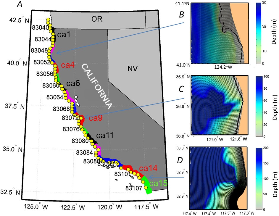
(A) Map of 15 SWAN grids along the California coast used in the study. Yellow dots denote the location of WIS boundary points used in the model simulations; station IDs are shown for every fourth boundary point. Example close-up views of the grids and bathymetry in the vicinity of (B) Trinidad, (C) Monterey Canyon, and (D) La Jolla Canyon display the great bathymetric and topographic variability that results in large spatial gradients of wave energy along California.
 In shallow water, the orbital motions of water particles induced by surface waves extend down to the seabed (see inset). The resulting wave-induced orbital velocities near the seabed are considered to be a representative measure of how waves influence the sea floor and as such are a focus of this study. The SWAN model calculates bottom orbital velocity (Uorb) as the maxima of the root mean square (rms) bottom velocity (Urms):
![]() (1)
(1)
where δ is the wave frequency; θ is the wave direction; k is the wave number (=2π⁄L) with L as the wavelength which in turn is related to the constant π, acceleration due to gravity (g = 9.81 m/s2), water depth d, and wave period, T; and E(δ, θ) is the wave energy density related to g, δ, θ, water density, and wave height (H). In essence, the orbital velocities are a function of three primary wave descriptors, namely the wave height, wave period, and wavelength.
Wave energy flux is the rate at which energy is transmitted in the direction of wave propagation across a vertical plane perpendicular to the direction of wave advance and extending throughout the water column (Demirbilik and Linwood, 2002). Assuming linear wave theory, the average energy flux per unit wave crest transmitted across a vertical plane and perpendicular to the direction of wave advance, also known as wave power P, may be expressed as
where E is the specific energy density = 1/8ρgH2, and Cg the group velocity which depends on relative water depth:
| for shallow water, d/L<1/20 (3) | |
| for transitional water, 1/20 < d/L <1/2 (4) | |
| for deep water, d/L>1/2 (5) |
Estimates of total P for all wave directions were calculated for each of the model domains, each season, and statistic (mean and top 5%). These data are not directly provided in downloadable files but can be computed with the relationships listed above.
Wave and wind data employed at model boundaries
Wave and wind data used as boundary conditions to the models run as part of this study were obtained from the Coastal and Hydraulics Laboratory (2013) Wave Information System (WIS) study. In that study, wave hind-casts were calculated with the numerical wave model WAM (Wave Prediction Model) Cycle 4.5.1C (Gunther and others, 1992; Komen and others, 1994) on a 0.25° grid (approximately 28 km at 37°N). Ten-meter height neutrally stable marine winds, compiled and analyzed by Oceanweather, Inc. (2012), were used as boundary conditions in the WAM model. It is worth noting that the basic scientific philosophy of SWAN and WAM are the same. The models use similar formulations for the source terms and both describe wave generation and evolution of the wave spectrum by solving the action balance equation. The main difference between the models is the numerical implementation and inclusion of additional nearshore processes (depth-induced breaking and triad wave-wave interactions) in the SWAN model.
Continuous hourly wave and wind parameter time-series provided by the WIS study and encompassing the 32 years from 1980 through 2011 were used to calculate seasonal (arithmetic) mean and extreme (arithmetic mean of highest 5%) conditions. Seasons were defined as: winter = December through February; spring = March through May; summer = June through August; and fall = September through November.
Chapter 3. Model calibration and validation
The ability of the model to accurately simulate wave propagation was tested by running the model forced with hourly wave parameters of the WIS database over a week long time period from 18-25 January 2010. The simulation period encompasses a large storm event when wave heights exceeded 9 m (e.g., CDIP Pt. Reyes buoy) and affected the entire California coast.
The ability of the model to reproduce observed wave conditions was evaluated with a skill score, where (Willmott 1981):
![]() (6)
(6)
where X is H , and the subscripts obs and mod indicate measured and modeled values, respectively. Over-bars indicate time-averaged values. The skill score ranges from 0 to 1, with a skill score of 1 indicating perfect agreement. The analysis is done over the entire simulated time-series.
Skill scores are quite good (>0.80, Table 2) at all sites evaluated. The mean values and standard deviations are also within reason of each other. While observations are not available within all grids, the high skill scores and lack of clear geographic trend in changes of the skill score suggest that model results in grids with no buoys are likely also reflective of true condtions.
Table 2. Skill scores and mean value statistics of modeled and observed significant wave heights. Comparison is for 18-25 January 2010. Mean values and standard deviations (shown in parenthesis) are rounded to the nearest 0.05m.
| NDBC ID | Owner/ operator |
Longitude (°W) |
Latitude (°N) |
Model grid | Skill | Model mean & std |
Observed mean & std |
|---|---|---|---|---|---|---|---|
| 46027 | NDBC | 124.381 | 41.85 | ca1 | 0.91 | 3.50 (1.20) | 3.65 (1.25) |
| 46237 | SCRIPPS | 122.599 | 37.781 | ca7 | 0.91 | 2.65 (1.10) | 3.20 (1.50) |
| 46240 | SCRIPPS | 121.907 | 36.626 | ca9 | 0.92 | 1.25 (0.60) | 1.45 (0.60) |
| 46236 | SCRIPPS | 121.947 | 36.761 | ca9 | 0.97 | 2.90 (1.35) | 2.90 (1.20) |
| 46215 | SCRIPPS | 120.86 | 35.204 | ca12 | 0.97 | 2.60 (1.30) | 2.65 (1.10) |
| 46223 | SCRIPPS | 117.767 | 33.458 | ca14 | 0.92 | 1.40 (0.90) | 1.70 (0.90) |
| 46222 | SCRIPPS | 118.317 | 33.618 | ca14 | 0.84 | 1.45 (1.00) | 2.00 (0.93) |
| 46221 | SCRIPPS | 118.633 | 33.854 | ca14 | 0.85 | 1.30 (0.95) | 1.90 (0.85) |
| 46231 | SCRIPPS | 117.37 | 32.748 | ca15 | 0.81 | 1.40 (0.65) | 2.00 (0.85) |
| 46225 | SCRIPPS | 117.393 | 32.93 | ca15 | 0.87 | 1.30 (0.65) | 1.70 (0.80) |
| 46241 | SCRIPPS | 117.292 | 33.003 | ca15 | 0.86 | 1.15 (0.60) | 1.50 (0.61) |
| 46224 | SCRIPPS | 117.471 | 33.179 | ca15 | 0.86 | 1.05 (0.50) | 1.45 (0.80) |
| 46242 | SCRIPPS | 117.44 | 33.22 | ca15 | 0.9 | 1.00 (0.50) | 1.25 (0.80) |
|
NDBC: National Data Buoy Center |
|||||||
Chapter 4. Summary of wave and seabed energetics
Wave heights and incident wave energy at the model boundaries
Mean and top 5% incident wave directions are all from the west to northwest along the open boundaries of the model grids (Figure 2). Mean incident wave directions range from 212° to 288°, whereas under extreme conditions of the top 5%, wave directions are more northerly ranging from 252° to 328°. The seasonal variation in mean incident wave directions is much smaller than those of extreme conditions: overall mean conditions vary by ±3° compared to ±11° for the averaged seasonal extreme directions. In northern California, summer extreme events originate from more northerly directions compared to storms during the remaining times of the year. In southern California south of Point Conception, incident storm waves are from nearly identical directions independent of the season (Figure 2B).
Figure 2. Seasonal wave heights and directions at model grid open boundaries.

(A) Mean and (B) extreme (top 5%) wave heights and associated directions for the WIS station located at the approximate mid-point of each grid are shown. [Click for larger version.]
Significant wave heights are smallest in summer and largest in winter, as expected. Mean summer conditions along the entire coast are 1.5 m ± 0.4 m whilst winter mean conditions are one meter higher with an average of 2.4 m ± 0.8 m. Seasonally averaged wave heights are greatest in northern California and smallest in Southern California (e.g., 3.3 m in north and less than 1.0 m in south during the winter season). A similar pattern exists for extreme conditions. Winter extremes are on average 6.3 m in the north and 2.0 m in the south. Similarly, averaged extreme summer wave heights decrease from 3.2 m in the north to just over 1 m in the south. Spring and fall conditions also show a decreasing trend with decreasing latitude and both experience significant wave heights on the order of 5.0 m in the north. Whereas the deceasing trend is consistent, spring significant wave heights are typically greater than fall significant wave heights along the central and southern portions of the State.
Seasonally averaged peak wave periods (not shown but listed in Table A1) are longest in winter (15 s ± 1 s) and shortest in summer (10 s ± 3 s). The difference between wave periods of extreme conditions and background mean conditions is less than 2 s for all seasons.
Wave power and near-bed wave-orbital velocities
Wave power, simulated with the SWAN model, shows substantial variation along the California coast and across the continental shelf. Similar to forcing conditions at the model boundaries (previous section), wave power (Equation 2) is greatest in the north part of the State and smallest in the south (shaded colors in Figures 3 through 6). Winter and fall seasons (Figure 3 and Figure 6) show the greatest difference between average ‘background’ and extreme conditions when wave power is as much as 5 times greater.
Figure 3. Winter (December-February) wave power along the inner margin of the California shelf.
(A) Mean and (B) extreme (top 5%) conditions.
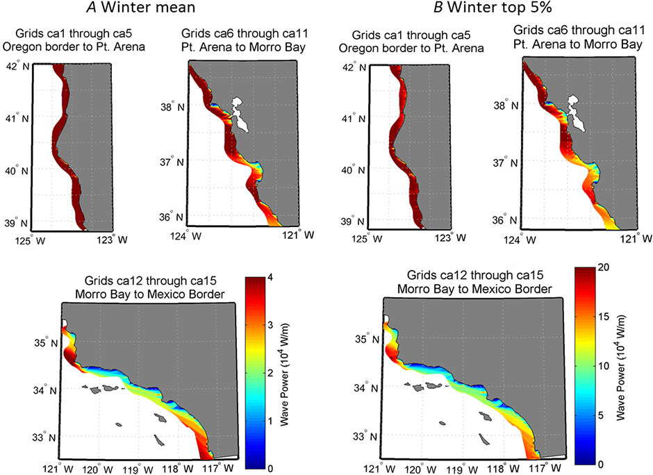
Figure 4. Spring (March-May) wave power along the inner margin of the California shelf.
(A) Mean and (B) extreme (top 5%) conditions.
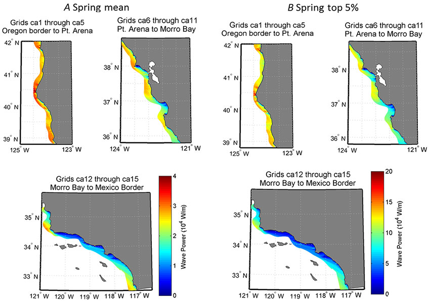
Figure 5. Summer (June-August) wave power along the inner margin of the California shelf.
(A) Mean and (B) extreme (top 5%) conditions.
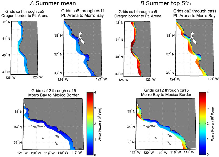
Figure 6. Fall (September-November) wave power along the inner margin of the California shelf.
(A) Mean and (B) extreme (top 5%) conditions.
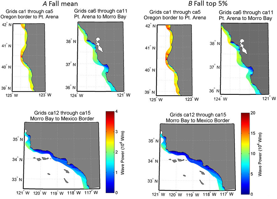
Near-bed wave-orbital velocities show similar patterns but are difficult to decipher at the scale offered in Figures 3 through 6. As an alternative, and because this methods summary is intended to provide an overview to the downloadable data rather than detailed analysis, seasonal and latitudinal patterns are evaluated on a per grid basis by obtaining average values at each of the 15 grids (Figures 7 and 8). This type of comparison shows that during extreme winter, spring, and fall conditions, wave power is much greater than average conditions during any other time of the year and extremes during the summer. In fact, summer extremes are only slightly greater than average spring and fall wave power. Similarly, near-bed wave-orbital velocities during extreme summer conditions are about equal to background spring and fall near bed disturbances. In a general sense, extreme conditions during spring and fall yield very similar near-bed disturbances, with maximum across shelf averaged near-bed wave-orbital velocities reaching approximately 1.1 m/s at the north end of the State.
Figure 7. Model grid-averaged wave and seabed energetics as a function of latitude. (A) Wave power, and (B) wave-orbital velocities. (C) Reference map showing locations for A and B.
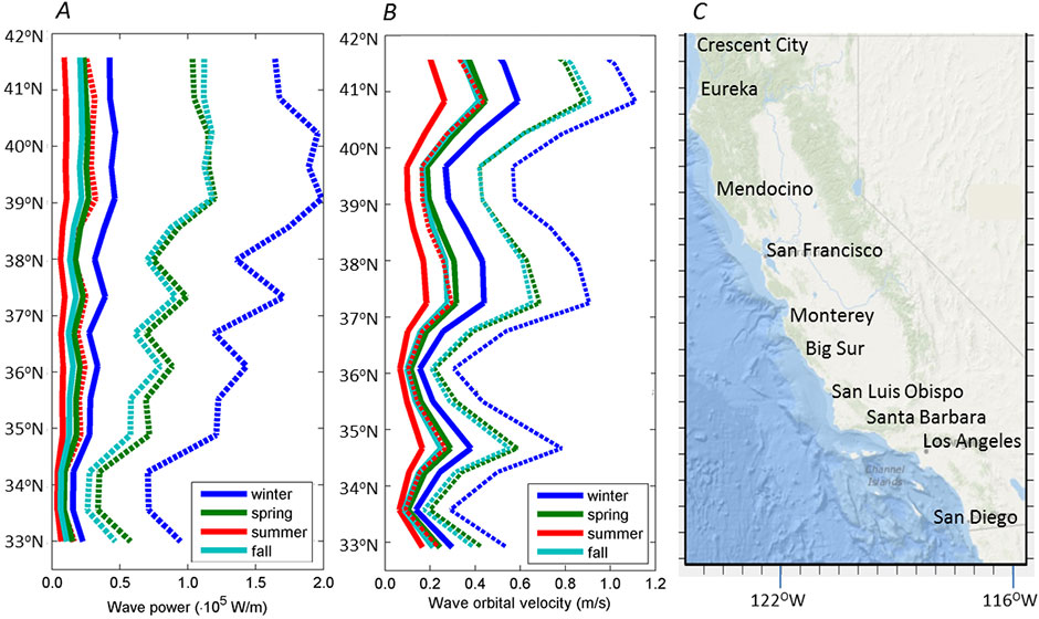
Figure 8. Seabed wave-orbital mean and standard deviation velocities of each grid separated by season for mean (gray squares) and top 5% (white squares) conditions. Note the variation in the scale of the vertical axes varies with latitude.
While these results do not address to what degree these wave motions impact the seabed, they do show that peak wave-induced wave-orbital velocities are more than twice the near-bed tidal current speeds and subtidal current speeds observed along California (for example, Sherwood and others, 1994; Steger and others, 1998; Noble and Ramp, 2000; Storlazzi and Jaffe, 2002, Xu and others, 2002; Storlazzi and others, 2003, Drake and others, 2005), supporting the conclusion that this is a wave-dominated shelf. These results suggest that benthic infauna and epifauna along this continental shelf are adapted to a dynamic hydrodynamic environment. Many of the deeper bedrock reefs are frequently subjected to 0.1-0.2 m/s wave-orbital velocities, and almost all of the shallow bedrock reefs on the inner most portions of the continental shelf (less than 10 m depth, generally less than 1 km from shore), except those in the lee of headlands, are frequently subjected to strong wave-orbital velocities (greater than 0.5 m/s). These shallow bedrock reefs along California typically host giant kelp forests, which are second only to tropical rainforests in biomass production per m2 (Mann, 1973), and thus the kelp plants and the ecosystem they support have developed in this wave-impacted environment. The spatial and temporal variability in frequency of elevated wave-orbital velocities likely plays into the life history of many organisms and the structure of their ecosystems (for example, species diversity), as suggested by Connell (1978). The community structure of numerous temperate water sessile organisms is influenced by spatial and temporal variations in wave energy similar to those described here. Large wave events have been shown to decrease kelp forest biomass (Graham et al., 1997), increase benthic macroalgae species richness (Wernberg and Goldberg, 2008), and cause mass mortality of nearshore fish species (Bodkin and others, 1987).
References Cited
Allan, J., and Komar, P.D., 2000. Are ocean wave heights increasing in the eastern North Pacific? EOS, Transactions of the American Geophysical Union, 81, 561-567.
Battjes, J., and Janssen, J., 1978. Energy loss and set-up due to breaking of random waves. In Proceedings 16th International Conference Coastal Engineering, ASCE, pp. 569-587.
Bodkin, J.L, VanBlaricom, G.R., and Jameson, R.J., 1987. Mortalities of kelp-forest fishes associated with large oceanic waves off central California: 1982-1983. Environmental Biology of Fishes, 18(1), 73-76.
Booij, N., Ris, R.C., and Holthuijsen, L.H., 1999. A third generation model for coastal regions, Part I – Model description and validation. Journal of Geophysical Research, 104(C4), 7649-7666.
Bromirski, P.D., Cayan, D.R., and Flick, R.E., 2005. Wave spectral energy variability in the Northeast Pacific. Journal of Geophysical Research, 110(C03005), doi:10.1029/2004JC002398.
Coastal and Hydraulics Laboratory, 2013. Wave Information Studies – Pacific data. Engineer Research and Development Center, US Army Corps of Engineers. [http://wis.usace.army.mil/hindcasts.shtml?dmn=pacWIS4]
Connell, J. H., 1978. Diversity in tropical rain forests and coral reefs. Science, 199, 1302–1310.
Demirbilik, Z., and Linwood, V.C. (2002). "Water wave mechanics," In: Coastal Engineering Manual, Part II-1 , Engineer Manual 1110-2-1100, U.S. Army Corps of Engineers, Washington, DC.
Drake, P., McManus, M.A., and Storlazzi, C.D., 2005. Local wind forcing of the Monterey Bay area inner shelf. Continental Shelf Research, 25, 397-417.
Garrison, T. 1996. Oceanography. An Invitation to Marine Science. Second Edition. Wadsworth Publishing Company.
Goodsell, P.J., and Connell, S.D., 2005. Historical configuration of habitat influences and the effects of the disturbance on mobile invertebrates. Marine Ecology Progress Series, 299, 79-87.
Graham, M.H., Harrold, C., Lisin, S., Light, K., Watanabe, J.M., and Foster, M.S., 1997. Population dynamics of giant kelp Macrocystis pyrifera along a wave exposure gradient. Marine Ecology Progress Series, 148, 269-279.
Griffen, J.D., Hemer, M.A., and Jones, B.G., 2008. Mobility of sediment grain size distributions on a wave dominated continental shelf, southeastern Australia. Marine Geology, 252, 13-23.
Gunther, H., Hasselmann, S., Janssen, P.A.E.M., 1992 Technical Report No. 4 WAM Model Cycle 4. Technical Report. [http://info.dkrz.de/forschung/reports/report4/wamh-1.html]
Hemer, M.A., 2006. The magnitude and frequency of combined flow bed shear stress as a measure of exposure on the Australian continental shelf. Continental Shelf Research, v. 26, p. 1258-1280.
Inman, D.L. and Jenkins, S.A., 1997. Changing wave climate and littoral drift. California and World Ocean, ’97, Conference Proceedings, chap. 73, 539-549.
Komen, G., Hasselmann, S, and Hasselmann, K., 1984. On the existence of a fully developed wind-sea spectrum. Journal of Physical Oceanography(14), pp. 1271-1285.
Komen, G.J, Cavaleri, L., Donelan, M., Hasselmann, K., Hasselmann, S. and Janssen, P.A.E.M., 1994. Dynamics and Modeling of Ocean Waves. Cambridge University Press, 532 p.
Mann, K.H., 1973. Seaweeds- their productivity and strategy for growth. Science, 182, 975-981.
National Data Buoy Center, 2006. Station 46042 – MONTEREY data. National Oceanic and Atmospheric Administration. [http://www.ndbc.noaa.gov/station_page.php?station=46042].
Noble, M.A., and Ramp, S.R., 2000. Subtidal currents over the central California slope: Evidence for offshore veering of the undercurrent and for direct, wind-driven slope currents. Deep-Sea Research II, 47, 871-906.
Oceanweather, Inc., 2012. MetOcean data. [http://www.oceanweather.com/metocean/]
Porter-Smith, R., Harris, P.T., Andersen, O.B., Coleman, R., Greensdale, D., and Jenkins, C.J., 2004. Classification of the Australian continental shelf based on predicted sediment threshold exceedance from tidal currents and swell waves. Marine Geology, 211, 1-20.
Ris, R.C., 1997. Spectral modeling of wind waves in coastal areas. Delft, The Netherlands, Ph.D. dissertation, Delft University of Technology, Department of Civil Engineering, Communications on Hydraulic and Geotechnical Engineering, Report No. 97-4.
Ris, R.C., Booij, N., and Holthuijsen, L.H., 1999. A third-generation wave model for coastal regions: Part II –Verification.: Journal of Geophysical Research, 104(C4), 7667-7682.
Roff, J.C., Taylor, M.E., and Laughren, J., 2003. Geo-physical approaches to the classification, delineation, and monitoring of marine habitats and their communities. Aquatic Conservation-Marine and Freshwater Ecosystems, 13, 77-90.
Seymour, R.J., Strange, R.R., Cayan, D.R. and Nathan, R.A., 1984. Influence of El Niños on California’s wave climate. Proceedings of the 19th Coastal Engineering Conference, American Society of Civil Engineers, 1, 577-592.
Seymour, R.J., 1998. Effects of El Niños on the West Coast wave climate. Shore and Beach, 66(3), 3-6.
Sherwood, C.R., Butman, B., Cacchione, D.A., Drake, D.E., Gross, T.F., Sternberg, R.W., Wiberg, P.L., and Williams, A.J. III, 1994. Sediment-transport events on the northern California continental shelf during the 1990-1991 STRESS experiment. Continental Shelf Research, 14, 1063-1100.
Snelgrove, P.V.R., and Butman, C.A., 1994. Animal-sediment relationships revisited – Cause versus effect. Oceanography and Marine Biology Annual Review, 32, 111-177.
Steger, J.M., Collins, C.A., Schwing, F.B., Noble, M., Garfield, N., and Steiner, M.T., 1998. An empirical model of the tidal currents in the Gulf of the Farallones. Deep-Sea Research II, 45, 1471-1505.
Storlazzi, C.D. and Griggs, G.B., 2000. The influence of El Niño-Southern Oscillation (ENSO) events on the evolution of central California’s shoreline. Geological Society of America Bulletin, 112(2), 236-249.
Storlazzi, C.D., and Jaffe, B.E., 2002. Flow and sediment suspension events on the inner shelf of central California. Marine Geology, 181(1-3), 195-213.
Storlazzi, C.D., McManus, M.A., and Figurski, J.D., 2003. Long-term high-frequency ADCP and temperature measurements along central California: Insights into upwelling and internal waves on the inner shelf. Continental Shelf Research, 23, 901-918.
Storlazzi, C.D., Reid, J.A., 2010. The influence of El Niño-Southern Oscillation (ENSO) cycles on wave-driven sea-floor sediment mobility along the central California continental margin. Contintental Shelf Researcch, 30, 1582-1599.
SWAN team. 2013. SWAN, Scientific and Technical documentation SWAN Cycle III version 70.91ABC, Delft Unvierstiy of Technology, The Netherlands. http://swanmodel.sourceforge.net/online_doc/swantech/swantech.html
Thrush, S.F., and Dayton, P.K., 2002. Disturbance to marine benthic habitats by trawling and dredging- implications for marine biodiversity. Annual Reviews of Ecology and Systematics, 33, 449-473.
Wernberg, T., and Goldberg, N., 2008. Short-term temporal dynamics of algal species in a subtidal kelp bed in relation to changes in environmental conditions and canopy biomass. Estuarine, Coastal and Shelf Science, 76, 265-272.
Xu., J.P., Noble, M., and Eittreim, S. L., 2002. Suspended sediment transport on the continental shelf near Davenport, California. Marine Geology, 181(1-3), 171-194.
Appendix A. Mean and top 5% wave conditions at each WIS station used as boundaries to the SWAN model
Table A-1. Mean boundary conditions derived from the WIS station data – winter and spring
| WIS ID | Latitude (°N) |
Longitude (°W) |
Depth (m) |
Winter (Dec-Feb) | Spring (Mar-May) | ||||||||
|---|---|---|---|---|---|---|---|---|---|---|---|---|---|
| Hs (m) |
Tp (s) |
Dm (°) |
Ua (m/s) |
Udir (°) |
Hs (m) |
Tp (s) |
Dm (°) |
Ua (m/s) |
Udir (°) |
||||
| 83037 | 42.50 | 124.67 | 227 | 3.3 | 14 | 272 | 9 | 200 | 2.5 | 12 | 284 | 8 | 309 |
| 83038 | 42.33 | 124.67 | 365 | 3.3 | 14 | 272 | 9 | 200 | 2.6 | 12 | 285 | 8 | 311 |
| 83039 | 42.17 | 124.50 | 148 | 3.1 | 14 | 273 | 9 | 200 | 2.5 | 12 | 285 | 8 | 312 |
| 83040 | 42.00 | 124.50 | 157 | 3.2 | 14 | 273 | 9 | 200 | 2.5 | 12 | 286 | 8 | 314 |
| 83041 | 41.83 | 124.42 | 193 | 3.1 | 14 | 274 | 9 | 199 | 2.5 | 12 | 287 | 8 | 316 |
| 83042 | 41.67 | 124.25 | 63 | 2.8 | 14 | 271 | 9 | 199 | 2.3 | 12 | 283 | 8 | 317 |
| 83043 | 41.50 | 124.25 | 77 | 3.0 | 14 | 275 | 9 | 199 | 2.4 | 12 | 287 | 8 | 319 |
| 83044 | 41.33 | 124.25 | 100 | 3.0 | 14 | 277 | 9 | 199 | 2.5 | 12 | 289 | 8 | 320 |
| 83045 | 41.17 | 124.25 | 107 | 3.0 | 14 | 279 | 9 | 199 | 2.4 | 12 | 291 | 8 | 322 |
| 83046 | 41.00 | 124.25 | 63 | 2.9 | 14 | 281 | 8 | 198 | 2.4 | 12 | 292 | 8 | 324 |
| 83047 | 40.83 | 124.42 | 260 | 3.1 | 14 | 281 | 8 | 201 | 2.6 | 12 | 294 | 8 | 323 |
| 83048 | 40.67 | 124.50 | 340 | 3.1 | 14 | 281 | 8 | 206 | 2.6 | 12 | 294 | 8 | 324 |
| 83049 | 40.50 | 124.5. | 128 | 3.1 | 14 | 280 | 8 | 214 | 2.6 | 12 | 293 | 8 | 324 |
| 83050 | 40.33 | 124.5. | 704 | 3.1 | 14 | 281 | 8 | 223 | 2.6 | 12 | 294 | 8 | 324 |
| 83051 | 40.17 | 124.42 | 477 | 3.1 | 14 | 281 | 7 | 237 | 2.5 | 12 | 292 | 7 | 324 |
| 83052 | 40.00 | 124.25 | 724 | 3.0 | 14 | 279 | 8 | 297 | 2.4 | 12 | 288 | 8 | 324 |
| 83053 | 39.83 | 124.00 | 170 | 2.8 | 14 | 277 | 6 | 352 | 2.2 | 12 | 285 | 6 | 322 |
| 83054 | 39.67 | 124.00 | 489 | 3.0 | 14 | 281 | 8 | 350 | 2.4 | 12 | 289 | 7 | 323 |
| 83055 | 39.50 | 124.00 | 574 | 3.0 | 14 | 282 | 8 | 350 | 2.5 | 12 | 292 | 7 | 323 |
| 83056 | 39.33 | 124.00 | 541 | 3.0 | 14 | 283 | 8 | 351 | 2.5 | 12 | 293 | 7 | 323 |
| 83057 | 39.17 | 123.92 | 247 | 3.0 | 14 | 283 | 6 | 354 | 2.5 | 12 | 293 | 6 | 323 |
| 83058 | 39.00 | 123.92 | 325 | 3.0 | 14 | 284 | 8 | 354 | 2.5 | 12 | 294 | 7 | 323 |
| 83059 | 38.83 | 123.75 | 120 | 2.8 | 14 | 280 | 7 | 350 | 2.3 | 12 | 290 | 7 | 323 |
| 83060 | 38.67 | 123.50 | 99 | 2.3 | 14 | 272 | 4 | 349 | 1.8 | 12 | 279 | 3 | 321 |
| 83061 | 38.50 | 123.42 | 134 | 2.7 | 14 | 279 | 7 | 345 | 2.2 | 12 | 288 | 7 | 322 |
| 83062 | 38.33 | 123.25 | 108 | 2.7 | 14 | 280 | 7 | 343 | 2.3 | 12 | 289 | 8 | 323 |
| 83063 | 38.17 | 123.17 | 99 | 2.7 | 14 | 282 | 7 | 342 | 2.3 | 12 | 291 | 7 | 323 |
| 83064 | 38.00 | 123.17 | 137 | 2.8 | 14 | 283 | 6 | 341 | 2.4 | 12 | 292 | 6 | 323 |
| 83065 | 37.83 | 122.92 | 72 | 2.5 | 14 | 280 | 6 | 339 | 2.1 | 12 | 288 | 6 | 324 |
| 83066 | 37.67 | 122.67 | 39 | 2.3 | 14 | 271 | 6 | 338 | 1.9 | 13 | 280 | 6 | 324 |
| 83067 | 37.50 | 122.67 | 72 | 2.3 | 14 | 277 | 6 | 338 | 2.0 | 12 | 286 | 6 | 324 |
| 83068 | 37.33 | 122.67 | 98 | 2.6 | 14 | 282 | 7 | 337 | 2.3 | 12 | 291 | 7 | 325 |
| 83069 | 37.17 | 122.67 | 191 | 2.7 | 14 | 286 | 7 | 336 | 2.4 | 12 | 295 | 8 | 325 |
| 83070 | 37.00 | 122.50 | 314 | 2.7 | 14 | 287 | 7 | 336 | 2.4 | 12 | 295 | 8 | 326 |
| 83071 | 36.92 | 122.25 | 454 | 2.4 | 14 | 283 | 7 | 338 | 2.1 | 12 | 289 | 8 | 326 |
| 83072 | 36.83 | 122.00 | 267 | 2.0 | 14 | 278 | 5 | 340 | 1.7 | 12 | 282 | 6 | 326 |
| 83073 | 36.67 | 122.17 | 1435 | 2.7 | 14 | 288 | 7 | 339 | 2.4 | 12 | 295 | 8 | 326 |
| 83074 | 36.50 | 122.17 | 1353 | 2.8 | 14 | 290 | 7 | 340 | 2.5 | 12 | 297 | 8 | 327 |
| 83075 | 36.33 | 122.00 | 203 | 2.7 | 14 | 290 | 7 | 341 | 2.4 | 12 | 297 | 8 | 327 |
| 83076 | 36.17 | 121.92 | 971 | 2.7 | 14 | 290 | 5 | 342 | 2.4 | 12 | 296 | 6 | 327 |
| 83077 | 36.00 | 121.75 | 1037 | 2.7 | 14 | 290 | 6 | 342 | 2.4 | 12 | 295 | 8 | 327 |
| 83078 | 35.83 | 121.67 | 849 | 2.7 | 14 | 291 | 6 | 342 | 2.4 | 12 | 296 | 7 | 327 |
| 83079 | 35.67 | 121.50 | 651 | 2.7 | 14 | 291 | 6 | 342 | 2.4 | 12 | 296 | 7 | 327 |
| 83080 | 35.50 | 121.25 | 434 | 2.6 | 14 | 289 | 6 | 342 | 2.3 | 13 | 294 | 7 | 327 |
| 83081 | 35.33 | 121.17 | 463 | 2.6 | 14 | 291 | 6 | 341 | 2.4 | 12 | 296 | 7 | 327 |
| 83082 | 35.17 | 121.00 | 399 | 2.6 | 14 | 291 | 6 | 340 | 2.3 | 13 | 296 | 8 | 326 |
| 83083 | 35.00 | 120.75 | 94 | 2.3 | 14 | 288 | 7 | 338 | 2.1 | 12 | 293 | 8 | 325 |
| 83084 | 34.83 | 120.92 | 313 | 2.6 | 14 | 293 | 7 | 338 | 2.4 | 12 | 299 | 8 | 325 |
| 83085 | 34.67 | 120.92 | 433 | 2.7 | 14 | 294 | 7 | 336 | 2.5 | 12 | 300 | 8 | 324 |
| 83086 | 34.50 | 120.75 | 438 | 2.6 | 14 | 294 | 7 | 331 | 2.5 | 12 | 300 | 8 | 321 |
| 83087 | 34.42 | 120.58 | 302 | 2.4 | 14 | 290 | 4 | 330 | 2.1 | 12 | 295 | 5 | 320 |
| 83088 | 34.33 | 120.42 | 363 | 2.1 | 14 | 288 | 5 | 325 | 1.9 | 12 | 291 | 6 | 315 |
| 83090 | 34.25 | 120.00 | 569 | 1.5 | 14 | 282 | 5 | 324 | 1.3 | 12 | 284 | 7 | 308 |
| 83091 | 34.25 | 119.75 | 301 | 1.1 | 13 | 278 | 5 | 330 | 1.0 | 11 | 279 | 6 | 306 |
| 83092 | 34.25 | 119.50 | 109 | 0.9 | 13 | 273 | 5 | 337 | 0.8 | 11 | 272 | 6 | 304 |
| 83093 | 34.17 | 119.42 | 160 | 1.0 | 13 | 279 | 4 | 331 | 0.9 | 12 | 278 | 5 | 300 |
| 83096 | 33.92 | 119.17 | 771 | 0.8 | 13 | 261 | 5 | 324 | 0.9 | 13 | 255 | 6 | 286 |
| 83099 | 33.83 | 118.67 | 802 | 0.9 | 13 | 263 | 5 | 326 | 1.0 | 13 | 255 | 5 | 272 |
| 83100 | 33.67 | 118.50 | 783 | 0.9 | 13 | 271 | 5 | 320 | 1.0 | 12 | 267 | 5 | 273 |
| 83101 | 33.58 | 118.25 | 534 | 0.9 | 13 | 272 | 4 | 316 | 0.9 | 11 | 268 | 4 | 279 |
| 83102 | 33.50 | 118.00 | 467 | 0.8 | 14 | 268 | 4 | 315 | 0.9 | 13 | 259 | 5 | 273 |
| 83103 | 33.33 | 117.92 | 672 | 0.7 | 13 | 258 | 4 | 313 | 0.8 | 13 | 250 | 5 | 280 |
| 83105 | 33.08 | 117.67 | 824 | 1.0 | 14 | 269 | 4 | 315 | 1.0 | 13 | 261 | 5 | 285 |
| 83107 | 32.75 | 117.50 | 848 | 1.1 | 14 | 276 | 5 | 317 | 1.2 | 13 | 269 | 5 | 293 |
| Minimum | 39 | 0.7 | 13 | 258 | 4 | 198 | 0.8 | 11 | 250 | 3 | 272 | ||
| Maximum | 1435 | 3.3 | 14 | 294 | 9 | 354 | 2.6 | 13 | 300 | 8 | 327 | ||
| Mean | 395 | 2.4 | 14 | 280 | 7 | 305 | 2.1 | 12 | 287 | 7 | 316 | ||
| Standard Deviation | 318 | 0.8 | 0.3 | 8 | 2 | 57 | 0.6 | 0.4 | 12 | 1 | 15 | ||
Table A-2. Mean boundary conditions derived from WIS station data – summer and fall
| WIS ID | Latitude (°N) |
Longitude (°W) |
Depth (m) |
Summer (Jun-Aug) | Fall (Sep-Nov) | ||||||||
|---|---|---|---|---|---|---|---|---|---|---|---|---|---|
| Hs (m) |
Tp (s) |
Dm (°) |
Ua (m/s) |
Udir (°) |
Hs (m) |
Tp (s) |
Dm (°) |
Ua (m/s) |
Udir (°) |
||||
| 83037 | 42.50 | 124.67 | 227 | 1.8 | 9 | 306 | 8 | 342 | 2.5 | 12 | 290 | 7 | 328 |
| 83038 | 42.33 | 124.67 | 365 | 1.8 | 10 | 308 | 8 | 341 | 2.5 | 12 | 291 | 7 | 329 |
| 83039 | 42.17 | 124.50 | 148 | 1.8 | 9 | 306 | 8 | 341 | 2.4 | 12 | 291 | 7 | 331 |
| 83040 | 42.00 | 124.50 | 157 | 1.8 | 9 | 307 | 8 | 341 | 2.4 | 12 | 292 | 7 | 332 |
| 83041 | 41.83 | 124.42 | 193 | 1.8 | 9 | 307 | 8 | 341 | 2.4 | 12 | 292 | 7 | 333 |
| 83042 | 41.67 | 124.25 | 63 | 1.6 | 9 | 302 | 8 | 341 | 2.1 | 12 | 288 | 7 | 334 |
| 83043 | 41.50 | 124.25 | 77 | 1.8 | 9 | 306 | 8 | 340 | 2.3 | 12 | 292 | 7 | 335 |
| 83044 | 41.33 | 124.25 | 100 | 1.9 | 9 | 309 | 8 | 340 | 2.3 | 12 | 294 | 7 | 336 |
| 83045 | 41.17 | 124.25 | 107 | 1.9 | 9 | 310 | 8 | 340 | 2.3 | 12 | 296 | 7 | 337 |
| 83046 | 41.00 | 124.25 | 63 | 1.9 | 9 | 312 | 8 | 340 | 2.3 | 12 | 298 | 7 | 338 |
| 83047 | 40.83 | 124.42 | 260 | 2.0 | 9 | 314 | 8 | 339 | 2.4 | 12 | 299 | 7 | 338 |
| 83048 | 40.67 | 124.50 | 340 | 2.0 | 9 | 314 | 8 | 338 | 2.4 | 12 | 299 | 7 | 337 |
| 83049 | 40.50 | 124.5 | 128 | 2.0 | 9 | 313 | 8 | 337 | 2.4 | 12 | 298 | 7 | 337 |
| 83050 | 40.33 | 124.50 | 704 | 2.0 | 9 | 311 | 8 | 336 | 2.4 | 12 | 299 | 7 | 337 |
| 83051 | 40.17 | 124.42 | 477 | 1.9 | 10 | 306 | 6 | 335 | 2.4 | 12 | 297 | 6 | 337 |
| 83052 | 40.00 | 124.25 | 724 | 1.7 | 10 | 298 | 7 | 333 | 2.2 | 12 | 293 | 7 | 336 |
| 83053 | 39.83 | 124.00 | 170 | 1.5 | 10 | 291 | 5 | 330 | 2.0 | 12 | 289 | 5 | 335 |
| 83054 | 39.67 | 124.00 | 489 | 1.7 | 10 | 298 | 7 | 330 | 2.3 | 12 | 294 | 6 | 335 |
| 83055 | 39.50 | 124.00 | 574 | 1.8 | 10 | 301 | 7 | 330 | 2.4 | 12 | 296 | 6 | 335 |
| 83056 | 39.33 | 124.00 | 541 | 1.8 | 10 | 303 | 7 | 329 | 2.4 | 12 | 297 | 6 | 335 |
| 83057 | 39.17 | 123.92 | 247 | 1.8 | 10 | 303 | 5 | 329 | 2.4 | 12 | 297 | 5 | 335 |
| 83058 | 39.00 | 123.92 | 325 | 1.9 | 10 | 304 | 6 | 328 | 2.4 | 12 | 298 | 6 | 334 |
| 83059 | 38.83 | 123.75 | 120 | 1.7 | 10 | 299 | 6 | 327 | 2.1 | 12 | 294 | 6 | 334 |
| 83060 | 38.67 | 123.50 | 99 | 1.2 | 11 | 280 | 3 | 326 | 1.6 | 12 | 281 | 3 | 333 |
| 83061 | 38.50 | 123.42 | 134 | 1.5 | 10 | 292 | 6 | 325 | 2.0 | 12 | 291 | 6 | 332 |
| 83062 | 38.33 | 123.25 | 108 | 1.6 | 10 | 293 | 6 | 325 | 2.0 | 12 | 292 | 6 | 332 |
| 83063 | 38.17 | 123.17 | 99 | 1.6 | 10 | 296 | 6 | 325 | 2.0 | 12 | 294 | 6 | 332 |
| 83064 | 38.00 | 123.17 | 137 | 1.7 | 10 | 298 | 5 | 325 | 2.1 | 12 | 296 | 5 | 332 |
| 83065 | 37.83 | 122.92 | 72 | 1.5 | 10 | 292 | 5 | 324 | 1.8 | 12 | 291 | 5 | 332 |
| 83066 | 37.67 | 122.67 | 39 | 1.3 | 11 | 285 | 5 | 324 | 1.7 | 13 | 282 | 5 | 332 |
| 83067 | 37.50 | 122.67 | 72 | 1.5 | 10 | 291 | 5 | 324 | 1.7 | 12 | 288 | 5 | 332 |
| 83068 | 37.33 | 122.67 | 98 | 1.7 | 10 | 295 | 6 | 324 | 2.0 | 12 | 293 | 6 | 332 |
| 83069 | 37.17 | 122.67 | 191 | 1.8 | 10 | 298 | 7 | 324 | 2.1 | 12 | 297 | 6 | 332 |
| 83070 | 37.00 | 122.50 | 314 | 1.8 | 10 | 298 | 7 | 324 | 2.1 | 12 | 297 | 7 | 332 |
| 83071 | 36.92 | 122.25 | 454 | 1.6 | 10 | 290 | 7 | 324 | 1.8 | 12 | 290 | 6 | 332 |
| 83072 | 36.83 | 122.00 | 267 | 1.2 | 11 | 279 | 5 | 323 | 1.4 | 13 | 282 | 5 | 332 |
| 83073 | 36.67 | 122.17 | 1435 | 1.7 | 10 | 296 | 7 | 324 | 2.1 | 12 | 297 | 6 | 332 |
| 83074 | 36.50 | 122.17 | 1353 | 1.8 | 10 | 298 | 7 | 323 | 2.1 | 12 | 299 | 6 | 332 |
| 83075 | 36.33 | 122.00 | 203 | 1.8 | 10 | 298 | 7 | 323 | 2.1 | 12 | 298 | 6 | 332 |
| 83076 | 36.17 | 121.92 | 971 | 1.7 | 10 | 296 | 5 | 323 | 2.1 | 12 | 298 | 5 | 332 |
| 83077 | 36.00 | 121.75 | 1037 | 1.7 | 10 | 294 | 6 | 322 | 2.1 | 12 | 297 | 6 | 332 |
| 83078 | 35.83 | 121.67 | 849 | 1.7 | 10 | 296 | 6 | 322 | 2.1 | 12 | 298 | 5 | 332 |
| 83079 | 35.67 | 121.50 | 651 | 1.7 | 10 | 295 | 6 | 322 | 2.1 | 12 | 298 | 6 | 332 |
| 83080 | 35.50 | 121.25 | 434 | 1.6 | 11 | 291 | 6 | 322 | 1.9 | 13 | 295 | 6 | 332 |
| 83081 | 35.33 | 121.17 | 463 | 1.7 | 10 | 294 | 6 | 322 | 2.0 | 12 | 297 | 5 | 332 |
| 83082 | 35.17 | 121.00 | 399 | 1.6 | 10 | 294 | 6 | 322 | 2.0 | 12 | 297 | 6 | 331 |
| 83083 | 35.00 | 120.75 | 94 | 1.5 | 10 | 292 | 7 | 321 | 1.7 | 12 | 294 | 6 | 330 |
| 83084 | 34.83 | 120.92 | 313 | 1.7 | 10 | 298 | 7 | 321 | 2.1 | 12 | 300 | 6 | 330 |
| 83085 | 34.67 | 120.92 | 433 | 1.8 | 10 | 299 | 7 | 321 | 2.1 | 12 | 301 | 6 | 329 |
| 83086 | 34.50 | 120.75 | 438 | 1.8 | 10 | 299 | 7 | 318 | 2.1 | 12 | 301 | 6 | 326 |
| 83087 | 34.42 | 120.58 | 302 | 1.5 | 10 | 292 | 4 | 317 | 1.8 | 12 | 295 | 4 | 324 |
| 83088 | 34.33 | 120.42 | 363 | 1.3 | 11 | 288 | 5 | 312 | 1.5 | 13 | 292 | 5 | 320 |
| 83090 | 34.25 | 120.00 | 569 | 0.8 | 10 | 279 | 6 | 303 | .09 | 12 | 283 | 5 | 314 |
| 83091 | 34.25 | 119.75 | 301 | 0.6 | 9 | 277 | 5 | 300 | 0.7 | 11 | 279 | 5 | 315 |
| 83092 | 34.25 | 119.50 | 109 | 0.6 | 11 | 252 | 4 | 297 | 0.6 | 12 | 261 | 4 | 316 |
| 83093 | 34.17 | 119.42 | 160 | 0.6 | 11 | 260 | 4 | 294 | 0.6 | 12 | 269 | 4 | 312 |
| 83096 | 33.92 | 119.17 | 771 | 0.8 | 13 | 224 | 5 | 279 | 0.7 | 13 | 234 | 4 | 301 |
| 83099 | 33.83 | 118.67 | 802 | 0.8 | 14 | 234 | 4 | 264 | 0.7 | 14 | 241 | 4 | 295 |
| 83100 | 33.67 | 118.50 | 783 | 0.7 | 13 | 254 | 4 | 266 | 0.7 | 13 | 259 | 4 | 292 |
| 83101 | 33.58 | 118.25 | 534 | 0.6 | 11 | 235 | 3 | 274 | 0.6 | 12 | 249 | 3 | 295 |
| 83102 | 33.50 | 118.00 | 467 | 0.7 | 13 | 221 | 4 | 269 | 0.7 | 13 | 234 | 4 | 291 |
| 83103 | 33.33 | 117.92 | 672 | 0.7 | 14 | 212 | 4 | 276 | 0.7 | 14 | 223 | 4 | 294 |
| 83105 | 33.08 | 117.67 | 824 | 0.8 | 14 | 227 | 4 | 282 | 0.8 | 14 | 238 | 4 | 298 |
| 83107 | 32.75 | 117.50 | 848 | 0.9 | 13 | 237 | 4 | 290 | 0.9 | 14 | 250 | 4 | 303 |
| Minimum | 39 | 0.6 | 9 | 212 | 3 | 264 | 0.6 | 11 | 223 | 3 | 291 | ||
| Maximum | 1435 | 2.0 | 14 | 314 | 8 | 342 | 2.5 | 14 | 301 | 7 | 338 | ||
| Mean | 395 | 1.5 | 10 | 288 | 6 | 320 | 1.8 | 12 | 286 | 6 | 327 | ||
| Standard Deviation | 318 | 0.4 | 1.3 | 25 | 1 | 20 | 0.6 | 0.6 | 19 | 1 | 13 | ||
Table A-3. Top 5% boundary conditions derived from WIS station data – winter and spring
| WIS ID | Latitude (°N) |
Longitude (°W) |
Depth (m) |
Winter (Dec-Feb) | Spring (Mar-May) | ||||||||
|---|---|---|---|---|---|---|---|---|---|---|---|---|---|
| Hs (m) |
Tp (s) |
Dm (°) |
Ua (m/s) |
Udir (°) |
Hs (m) |
Tp (s) |
Dm (°) |
Ua (m/s) |
Udir (°) |
||||
| 83037 | 42.50 | 124.67 | 227 | 6.3 | 15 | 258 | 13 | 217 | 5.1 | 14 | 273 | 11 | 248 |
| 83038 | 42.33 | 124.67 | 365 | 6.3 | 15 | 259 | 13 | 217 | 5.1 | 14 | 274 | 11 | 252 |
| 83039 | 42.17 | 124.50 | 148 | 6.1 | 15 | 260 | 13 | 219 | 4.9 | 14 | 274 | 11 | 255 |
| 83040 | 42.00 | 124.50 | 157 | 6.1 | 15 | 261 | 13 | 219 | 5.0 | 14 | 276 | 11 | 259 |
| 83041 | 41.83 | 124.42 | 193 | 6.0 | 15 | 263 | 13 | 221 | 4.9 | 14 | 277 | 11 | 264 |
| 83042 | 41.67 | 124.25 | 63 | 5.5 | 15 | 260 | 12 | 219 | 4.5 | 14 | 272 | 11 | 258 |
| 83043 | 41.50 | 124.25 | 77 | 5.7 | 15 | 265 | 12 | 226 | 4.7 | 14 | 279 | 11 | 277 |
| 83044 | 41.33 | 124.25 | 100 | 5.7 | 15 | 268 | 12 | 232 | 4.8 | 14 | 283 | 11 | 290 |
| 83045 | 41.17 | 124.25 | 107 | 5.7 | 15 | 272 | 12 | 235 | 4.7 | 14 | 287 | 11 | 299 |
| 83046 | 41.00 | 124.25 | 63 | 5.5 | 15 | 276 | 12 | 243 | 4.7 | 14 | 290 | 12 | 309 |
| 83047 | 40.83 | 124.42 | 260 | 5.9 | 15 | 274 | 12 | 242 | 5.0 | 14 | 292 | 12 | 312 |
| 83048 | 40.67 | 124.50 | 340 | 6.0 | 15 | 272 | 12 | 242 | 5.0 | 14 | 293 | 12 | 314 |
| 83049 | 40.50 | 124.50 | 128 | 5.9 | 15 | 270 | 12 | 243 | 5.0 | 14 | 291 | 12 | 315 |
| 83050 | 40.33 | 124.50 | 704 | 6.1 | 15 | 272 | 12 | 243 | 5.0 | 14 | 292 | 12 | 315 |
| 83051 | 40.17 | 124.42 | 477 | 6.0 | 15 | 271 | 9 | 241 | 4.9 | 14 | 288 | 9 | 306 |
| 83052 | 40.00 | 124.25 | 724 | 5.9 | 15 | 269 | 11 | 236 | 4.8 | 14 | 282 | 10 | 297 |
| 83053 | 39.83 | 124.00 | 170 | 5.5 | 15 | 267 | 8 | 233 | 4.5 | 14 | 278 | 7 | 288 |
| 83054 | 39.67 | 124.00 | 489 | 5.8 | 15 | 272 | 11 | 241 | 4.8 | 14 | 286 | 11 | 305 |
| 83055 | 39.50 | 124.00 | 574 | 5.9 | 15 | 273 | 11 | 246 | 4.9 | 14 | 289 | 11 | 310 |
| 83056 | 39.33 | 124.00 | 541 | 5.9 | 15 | 274 | 11 | 248 | 4.9 | 14 | 291 | 11 | 314 |
| 83057 | 39.17 | 123.92 | 247 | 5.8 | 15 | 275 | 9 | 249 | 4.8 | 14 | 291 | 9 | 312 |
| 83058 | 39.00 | 123.92 | 325 | 5.8 | 15 | 275 | 11 | 250 | 4.9 | 14 | 292 | 11 | 316 |
| 83059 | 38.83 | 123.75 | 120 | 5.4 | 15 | 269 | 11 | 245 | 4.5 | 14 | 286 | 11 | 312 |
| 83060 | 38.67 | 123.50 | 99 | 4.8 | 15 | 260 | 5 | 227 | 3.7 | 14 | 270 | 5 | 280 |
| 83061 | 38.50 | 123.42 | 134 | 5.3 | 15 | 269 | 11 | 244 | 4.3 | 14 | 282 | 11 | 307 |
| 83062 | 38.33 | 123.25 | 108 | 5.3 | 15 | 271 | 10 | 252 | 4.4 | 14 | 284 | 11 | 314 |
| 83063 | 38.17 | 123.17 | 99 | 5.2 | 15 | 274 | 10 | 261 | 4.4 | 14 | 288 | 11 | 318 |
| 83064 | 38.00 | 123.17 | 137 | 5.5 | 16 | 276 | 8 | 265 | 4.7 | 14 | 290 | 8 | 319 |
| 83065 | 37.83 | 122.92 | 72 | 4.8 | 15 | 273 | 8 | 261 | 4.0 | 14 | 283 | 8 | 314 |
| 83066 | 37.67 | 122.67 | 39 | 4.5 | 15 | 262 | 8 | 262 | 3.7 | 14 | 275 | 8 | 316 |
| 83067 | 37.50 | 122.67 | 72 | 4.5 | 15 | 266 | 8 | 267 | 3.8 | 13 | 281 | 9 | 320 |
| 83068 | 37.33 | 122.67 | 98 | 5.0 | 15 | 274 | 10 | 279 | 4.3 | 14 | 289 | 11 | 325 |
| 83069 | 37.17 | 122.67 | 191 | 5.3 | 15 | 280 | 11 | 289 | 4.6 | 14 | 295 | 12 | 328 |
| 83070 | 37.00 | 122.50 | 314 | 5.3 | 15 | 280 | 11 | 293 | 4.6 | 14 | 295 | 12 | 329 |
| 83071 | 36.92 | 122.25 | 454 | 4.8 | 15 | 274 | 10 | 287 | 4.0 | 13 | 287 | 12 | 324 |
| 83072 | 36.83 | 122.00 | 267 | 4.2 | 15 | 269 | 7 | 274 | 3.4 | 14 | 277 | 8 | 314 |
| 83073 | 36.67 | 122.17 | 1435 | 5.3 | 15 | 283 | 10 | 298 | 4.6 | 14 | 295 | 12 | 327 |
| 83074 | 36.50 | 122.17 | 1353 | 5.4 | 15 | 285 | 10 | 301 | 4.7 | 14 | 298 | 12 | 327 |
| 83075 | 36.33 | 122.00 | 203 | 5.2 | 15 | 285 | 10 | 304 | 4.6 | 14 | 298 | 12 | 327 |
| 83076 | 36.17 | 121.92 | 971 | 5.3 | 15 | 285 | 8 | 303 | 4.6 | 14 | 296 | 9 | 326 |
| 83077 | 36.00 | 121.75 | 1037 | 5.2 | 16 | 285 | 9 | 303 | 4.5 | 14 | 295 | 11 | 326 |
| 83078 | 35.83 | 121.67 | 849 | 5.3 | 16 | 286 | 9 | 306 | 4.6 | 14 | 297 | 10 | 326 |
| 83079 | 35.67 | 121.50 | 651 | 5.2 | 16 | 286 | 9 | 307 | 4.5 | 14 | 297 | 11 | 326 |
| 83080 | 35.50 | 121.25 | 434 | 5.0 | 16 | 284 | 9 | 304 | 4.3 | 14 | 294 | 11 | 326 |
| 83081 | 35.33 | 121.17 | 463 | 5.1 | 16 | 287 | 9 | 308 | 4.5 | 14 | 296 | 10 | 326 |
| 83082 | 35.17 | 121.00 | 399 | 5.1 | 16 | 287 | 10 | 310 | 4.4 | 14 | 297 | 12 | 327 |
| 83083 | 35.00 | 120.75 | 94 | 4.6 | 15 | 283 | 10 | 308 | 4.0 | 14 | 292 | 12 | 324 |
| 83084 | 34.83 | 120.92 | 313 | 5.2 | 15 | 290 | 10 | 313 | 4.6 | 14 | 300 | 12 | 326 |
| 83085 | 34.67 | 120.92 | 433 | 5.2 | 15 | 292 | 10 | 315 | 4.7 | 14 | 302 | 12 | 326 |
| 83086 | 34.50 | 120.75 | 438 | 5.2 | 15 | 292 | 10 | 313 | 4.6 | 14 | 302 | 12 | 322 |
| 83087 | 34.42 | 120.58 | 302 | 4.6 | 15 | 286 | 6 | 310 | 4.0 | 14 | 293 | 7 | 318 |
| 83088 | 34.33 | 120.42 | 363 | 4.2 | 15 | 282 | 7 | 304 | 3.5 | 14 | 288 | 8 | 313 |
| 83090 | 34.25 | 120.00 | 569 | 3.3 | 15 | 278 | 8 | 299 | 2.7 | 13 | 282 | 11 | 306 |
| 83091 | 34.25 | 119.75 | 301 | 2.7 | 15 | 275 | 8 | 298 | 2.2 | 12 | 278 | 10 | 303 |
| 83092 | 34.25 | 119.5 | 109 | 2.2 | 14 | 271 | 8 | 297 | 1.9 | 10 | 275 | 10 | 299 |
| 83093 | 34.17 | 119.42 | 160 | 2.3 | 14 | 278 | 7 | 301 | 2.0 | 12 | 280 | 9 | 299 |
| 83096 | 33.92 | 119.17 | 771 | 2.2 | 11 | 252 | 9 | 273 | 2.0 | 8 | 265 | 11 | 280 |
| 83099 | 33.83 | 118.67 | 802 | 2.4 | 11 | 259 | 8 | 276 | 2.2 | 9 | 262 | 10 | 268 |
| 83100 | 33.67 | 118.50 | 783 | 2.5 | 12 | 269 | 9 | 282 | 2.3 | 9 | 271 | 10 | 270 |
| 83101 | 33.58 | 118.25 | 534 | 2.2 | 13 | 271 | 6 | 283 | 2.0 | 9 | 273 | 8 | 276 |
| 83102 | 33.50 | 118.00 | 467 | 2.1 | 12 | 266 | 8 | 274 | 1.9 | 10 | 270 | 9 | 270 |
| 83103 | 33.33 | 117.92 | 672 | 2.0 | 10 | 257 | 9 | 271 | 1.9 | 9 | 267 | 9 | 276 |
| 83105 | 33.08 | 117.67 | 824 | 2.5 | 12 | 267 | 9 | 279 | 2.3 | 9 | 274 | 9 | 282 |
| 83107 | 32.75 | 117.50 | 848 | 2.8 | 12 | 271 | 9 | 286 | 2.6 | 10 | 277 | 10 | 291 |
| Minimum | 39 | 2.0 | 10 | 252 | 5 | 217 | 1.9 | 8 | 262 | 5 | 248 | ||
| Maximum | 1435 | 6.3 | 16 | 292 | 13 | 315 | 5.1 | 14 | 302 | 12 | 329 | ||
| Mean | 395 | 4.8 | 15 | 273 | 10 | 269 | 4.1 | 13 | 285 | 10 | 304 | ||
| Standard Deviation | 318 | 1.3 | 1.3 | 9.0 | 2.0 | 31 | 1.0 | 1.7 | 10 | 2 | 23 | ||
Table A-4. Top 5% boundary conditions derived from WIS station data – summer and fall
| WIS ID | Latitude (°N) |
Longitude (°W) |
Depth (m) |
Summer (Jun-Aug) | Fall (Sep-Nov) | ||||||||
|---|---|---|---|---|---|---|---|---|---|---|---|---|---|
| Hs (m) |
Tp (s) |
Dm (°) |
Ua (m/s) |
Udir (°) |
Hs (m) |
Tp (s) |
Dm (°) |
Ua (m/s) |
Udir (°) |
||||
| 83037 | 42.50 | 124.67 | 227 | 3.2 | 10 | 316 | 13 | 349 | 5.4 | 14 | 276 | 11 | 244 |
| 83038 | 42.33 | 124.67 | 365 | 3.3 | 10 | 319 | 13 | 350 | 5.4 | 14 | 277 | 11 | 247 |
| 83039 | 42.17 | 124.50 | 148 | 3.2 | 10 | 314 | 13 | 349 | 5.2 | 14 | 277 | 11 | 249 |
| 83040 | 42.00 | 124.50 | 157 | 3.3 | 10 | 317 | 14 | 349 | 5.2 | 14 | 279 | 11 | 252 |
| 83041 | 41.83 | 124.42 | 193 | 3.3 | 10 | 317 | 14 | 349 | 5.1 | 14 | 280 | 11 | 257 |
| 83042 | 41.67 | 124.25 | 63 | 2.8 | 10 | 307 | 14 | 347 | 4.6 | 14 | 274 | 11 | 251 |
| 83043 | 41.50 | 124.25 | 77 | 3.2 | 10 | 315 | 14 | 349 | 4.9 | 14 | 280 | 11 | 265 |
| 83044 | 41.33 | 124.25 | 100 | 3.4 | 10 | 318 | 14 | 349 | 4.9 | 14 | 283 | 10 | 275 |
| 83045 | 41.17 | 124.25 | 107 | 3.4 | 9 | 320 | 14 | 349 | 4.8 | 14 | 287 | 10 | 284 |
| 83046 | 41.00 | 124.25 | 63 | 3.5 | 9 | 322 | 15 | 349 | 4.8 | 14 | 289 | 10 | 294 |
| 83047 | 40.83 | 124.42 | 260 | 3.7 | 10 | 326 | 14 | 349 | 5.1 | 14 | 292 | 10 | 300 |
| 83048 | 40.67 | 124.50 | 340 | 3.8 | 10 | 328 | 14 | 348 | 5.1 | 14 | 293 | 11 | 303 |
| 83049 | 40.50 | 124.50 | 128 | 3.7 | 10 | 326 | 14 | 347 | 5.0 | 14 | 291 | 10 | 304 |
| 83050 | 40.33 | 124.50 | 704 | 3.7 | 10 | 325 | 14 | 346 | 5.1 | 14 | 293 | 10 | 305 |
| 83051 | 40.17 | 124.42 | 477 | 3.4 | 10 | 317 | 11 | 344 | 5.0 | 14 | 291 | 8 | 300 |
| 83052 | 40.00 | 124.25 | 724 | 3.0 | 10 | 305 | 12 | 340 | 4.8 | 15 | 287 | 9 | 290 |
| 83053 | 39.83 | 124.00 | 170 | 2.6 | 11 | 296 | 8 | 336 | 4.4 | 15 | 283 | 6 | 286 |
| 83054 | 39.67 | 124.00 | 489 | 3.0 | 10 | 306 | 11 | 337 | 4.8 | 15 | 290 | 9 | 300 |
| 83055 | 39.50 | 124.00 | 574 | 3.2 | 10 | 310 | 11 | 338 | 4.9 | 14 | 293 | 9 | 308 |
| 83056 | 39.33 | 124.00 | 541 | 3.3 | 10 | 313 | 11 | 338 | 4.9 | 14 | 295 | 9 | 311 |
| 83057 | 39.17 | 123.92 | 247 | 3.2 | 10 | 311 | 9 | 337 | 4.8 | 14 | 295 | 8 | 313 |
| 83058 | 39.00 | 123.92 | 325 | 3.3 | 10 | 313 | 11 | 337 | 4.8 | 14 | 296 | 9 | 314 |
| 83059 | 38.83 | 123.75 | 120 | 3.0 | 10 | 308 | 11 | 336 | 4.3 | 14 | 290 | 9 | 312 |
| 83060 | 38.67 | 123.50 | 99 | 2.0 | 11 | 289 | 5 | 333 | 3.5 | 14 | 276 | 4 | 293 |
| 83061 | 38.50 | 123.42 | 134 | 2.7 | 11 | 300 | 11 | 334 | 4.1 | 14 | 287 | 9 | 309 |
| 83062 | 38.33 | 123.25 | 108 | 2.8 | 10 | 301 | 11 | 334 | 4.1 | 14 | 289 | 9 | 315 |
| 83063 | 38.17 | 123.17 | 99 | 2.9 | 10 | 303 | 10 | 334 | 4.2 | 14 | 292 | 9 | 321 |
| 83064 | 38.00 | 123.17 | 137 | 3.0 | 10 | 306 | 8 | 335 | 4.5 | 14 | 294 | 7 | 324 |
| 83065 | 37.83 | 122.92 | 72 | 2.5 | 11 | 298 | 8 | 334 | 3.9 | 15 | 288 | 7 | 320 |
| 83066 | 37.67 | 122.67 | 39 | 2.3 | 11 | 293 | 9 | 334 | 3.5 | 15 | 278 | 7 | 322 |
| 83067 | 37.50 | 122.67 | 72 | 2.6 | 10 | 300 | 9 | 334 | 3.4 | 13 | 286 | 8 | 326 |
| 83068 | 37.33 | 122.67 | 98 | 2.9 | 10 | 304 | 11 | 334 | 3.9 | 14 | 293 | 9 | 329 |
| 83069 | 37.17 | 122.67 | 191 | 3.2 | 10 | 308 | 12 | 335 | 4.3 | 14 | 298 | 10 | 332 |
| 83070 | 37.00 | 122.50 | 314 | 3.2 | 10 | 307 | 12 | 334 | 4.2 | 14 | 298 | 10 | 332 |
| 83071 | 36.92 | 122.25 | 454 | 2.7 | 10 | 299 | 12 | 332 | 3.6 | 14 | 291 | 10 | 329 |
| 83072 | 36.83 | 122.00 | 267 | 2.1 | 10 | 289 | 8 | 330 | 2.9 | 14 | 282 | 7 | 323 |
| 83073 | 36.67 | 122.17 | 1435 | 3.1 | 10 | 305 | 11 | 331 | 4.2 | 14 | 298 | 10 | 332 |
| 83074 | 36.50 | 122.17 | 1353 | 3.2 | 10 | 307 | 11 | 331 | 4.4 | 14 | 301 | 10 | 332 |
| 83075 | 36.33 | 122.00 | 203 | 3.1 | 10 | 306 | 11 | 329 | 4.4 | 14 | 301 | 10 | 332 |
| 83076 | 36.17 | 121.92 | 971 | 3.0 | 10 | 305 | 8 | 329 | 4.3 | 14 | 301 | 8 | 332 |
| 83077 | 36.00 | 121.75 | 1037 | 2.9 | 10 | 303 | 10 | 328 | 4.2 | 15 | 300 | 9 | 332 |
| 83078 | 35.83 | 121.67 | 849 | 3.0 | 10 | 304 | 9 | 328 | 4.3 | 14 | 301 | 9 | 333 |
| 83079 | 35.67 | 121.50 | 651 | 3.0 | 10 | 304 | 10 | 328 | 4.2 | 15 | 301 | 9 | 333 |
| 83080 | 35.50 | 121.25 | 434 | 2.7 | 11 | 300 | 10 | 328 | 4.0 | 15 | 298 | 9 | 333 |
| 83081 | 35.33 | 121.17 | 463 | 2.9 | 11 | 302 | 9 | 328 | 4.1 | 15 | 301 | 9 | 333 |
| 83082 | 35.17 | 121.00 | 399 | 2.8 | 11 | 302 | 10 | 328 | 4.0 | 14 | 301 | 10 | 333 |
| 83083 | 35.00 | 120.75 | 94 | 2.5 | 10 | 299 | 11 | 327 | 3.5 | 14 | 296 | 10 | 331 |
| 83084 | 34.83 | 120.92 | 313 | 3.0 | 10 | 306 | 10 | 327 | 4.2 | 14 | 304 | 10 | 333 |
| 83085 | 34.67 | 120.92 | 433 | 3.0 | 10 | 308 | 11 | 327 | 4.2 | 14 | 306 | 10 | 332 |
| 83086 | 34.50 | 120.75 | 438 | 3.0 | 10 | 307 | 11 | 324 | 4.2 | 14 | 305 | 10 | 329 |
| 83087 | 34.42 | 120.58 | 302 | 2.5 | 10 | 300 | 7 | 322 | 3.6 | 14 | 298 | 6 | 327 |
| 83088 | 34.33 | 120.42 | 363 | 2.1 | 10 | 295 | 8 | 317 | 3.1 | 14 | 294 | 7 | 323 |
| 83090 | 34.25 | 120.00 | 569 | 1.6 | 9 | 286 | 10 | 309 | 2.1 | 13 | 286 | 9 | 317 |
| 83091 | 34.25 | 119.75 | 301 | 1.3 | 8 | 281 | 9 | 306 | 1.7 | 12 | 282 | 9 | 317 |
| 83092 | 34.25 | 119.50 | 109 | 1.1 | 8 | 275 | 8 | 303 | 1.4 | 11 | 278 | 8 | 315 |
| 83093 | 34.17 | 119.42 | 160 | 1.2 | 9 | 280 | 7 | 300 | 1.5 | 11 | 283 | 7 | 314 |
| 83096 | 33.92 | 119.17 | 771 | 1.3 | 9 | 255 | 9 | 280 | 1.5 | 10 | 267 | 9 | 299 |
| 83099 | 33.83 | 118.67 | 802 | 1.4 | 10 | 256 | 7 | 265 | 1.6 | 10 | 265 | 8 | 295 |
| 83100 | 33.67 | 118.50 | 783 | 1.4 | 7 | 270 | 7 | 268 | 1.6 | 9 | 275 | 8 | 294 |
| 83101 | 33.58 | 118.25 | 534 | 1.2 | 8 | 265 | 5 | 275 | 1.5 | 9 | 272 | 6 | 296 |
| 83102 | 33.50 | 118.00 | 467 | 1.2 | 11 | 251 | 6 | 269 | 1.4 | 11 | 266 | 7 | 290 |
| 83103 | 33.33 | 117.92 | 672 | 1.2 | 12 | 239 | 6 | 277 | 1.4 | 11 | 259 | 7 | 291 |
| 83105 | 33.08 | 117.67 | 824 | 1.4 | 12 | 259 | 6 | 284 | 1.7 | 11 | 272 | 8 | 298 |
| 83107 | 32.75 | 117.50 | 848 | 1.5 | 11 | 269 | 7 | 294 | 1.9 | 11 | 279 | 8 | 305 |
| Minimum | 39 | 1.1 | 7 | 239 | 5 | 265 | 1.4 | 9 | 259 | 4 | 244 | ||
| Maximum | 1435 | 3.8 | 12 | 328 | 15 | 350 | 5.4 | 15 | 306 | 11 | 333 | ||
| Mean | 395 | 2.7 | 10 | 300 | 10 | 327 | 3.9 | 14 | 288 | 9 | 307 | ||
| Standard Deviation | 318 | 0.8 | 0.8 | 19 | 3 | 22 | 1.2 | 1.5 | 11 | 1 | 25 | ||
Figure A-1. Mean and extreme (top 5%) wave heights at each WIS station used as boundaries to the SWAN model. Standard deviations are shown with the vertical bars.
Figure A-2. Mean and extreme (top 5%) wave heights at each WIS station used as boundaries to the SWAN model. Standard deviations are shown with the vertical bars.
Figure A-3. Mean and extreme (top 5%) wave heights at each WIS station used as boundaries to the SWAN model. Standard deviations are shown with the vertical bars.
Figure A-4. Mean and extreme (top 5%) wave heights at each WIS station used as boundaries to the SWAN model. Standard deviations are shown with the vertical bars.
Figure A-5. Mean and extreme (top 5%) wave heights at each WIS station used as boundaries to the SWAN model. Standard deviations are shown with the vertical bars.
Figure A-6. Mean and extreme (top 5%) wave heights at each WIS station used as boundaries to the SWAN model. Standard deviations are shown with the vertical bars.
Figure A-7. Mean and extreme (top 5%) wave heights at each WIS station used as boundaries to the SWAN model. Standard deviations are shown with the vertical bars.
Conversion Factors
| Multiply | By | To obtain |
|---|---|---|
| Length | ||
| centimeter (cm) | 0.3937 | inch (in.) |
| millimeter (mm) | 0.03937 | inch (in.) |
| meter (m) | 3.281 | foot (ft) |
| kilometer (km) | 0.6214 | mile (mi) |
| kilometer (km) | 0.54 | mile, nautical (nmi) |
| meter (m) | 1.094 | yard (yd) |
Suggested citation: Erikson, Li H., Storlazzi, Curt D., and Golden, Nadine E., 2014. "Modeling Wave and Seabed Energetics on the California Continental Shelf:" Methods summary to accompany U. S. Geological Survey data set XXX, Wave and Orbital Velocity Model Data on the California Continental Shelf. doi:10.5066/F7125QNQ